Shelved indefinitely.
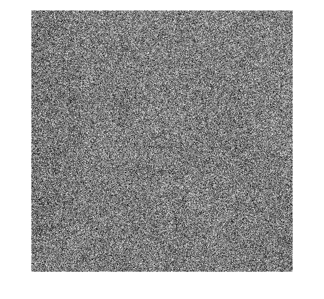
In high radiation environments, CMOS sensors can be locally saturated when struck with high-energy particles. This appears to an observer as a white pixel. When radiation levels become very high, saturated pixels become the dominant feature of the image. To an observer, this may make the image hard to read, and I believed a method to reject monochromatic noises would have utility.
In this method demonstration I will only consider the case of monochromatic noise applied to an image, with no leakage to other intensities. I shall also expect the noise present in the system… $$ \eta = \frac{n_{corrupted}}{n_{total}} > 0.005 $$ As I found detection of error frequencies to be challenging at lower levels.
I begin by defining the given image as an 8-bit grayscale, represented as matrix I. We can then define a perfect, error-free image as Io. We also are able to define our reconstructed image as Ir. The image will be X by Y pixels.
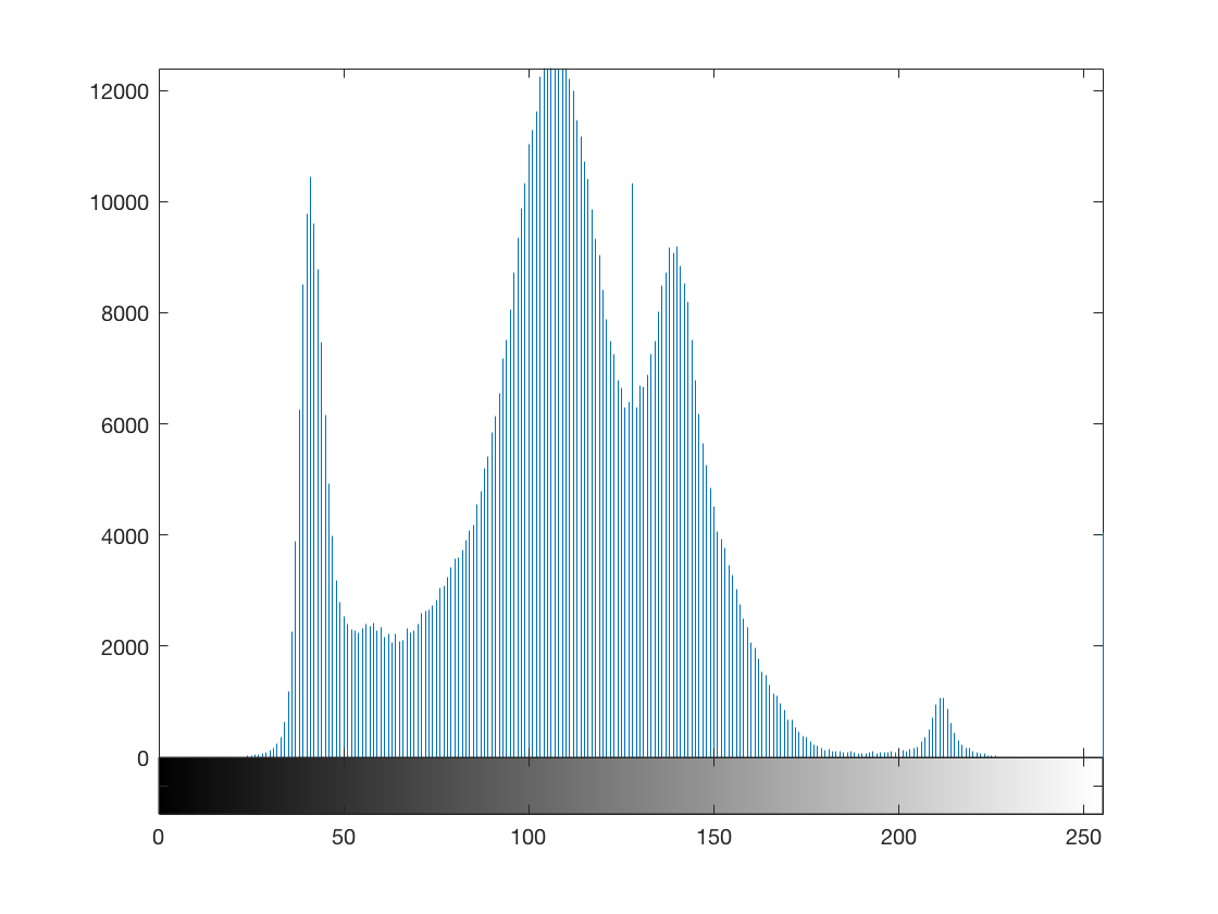
We begin by classifying what intensity our noises operate at. We take the second derivative of the image histogram.
$$ D(I,r) = \frac{\partial^2}{\partial r^2} \Bigg ( \int^{X}_{0} \int^{Y}_{0} \delta(I(x,y)-r)\mathrm{d}y\mathrm{d}x \Bigg )$$
Or, for the discrete case;
$$ D(I,r) = \nabla_{r} \nabla_{r} \sum^{X}_{i=0} \sum^{Y}_{j=0} \delta_ {{\bf{I}}_{i,j},r} $$
Where the nabla symbol represents a finite difference.
By inspection we should see that any monochromatic noises become sharp peaks in a histogram, which on taking the second derivative become amplified as abnormal features, even in the case of low (~2%) corruption.
In reality though, our data-set is not continuous, we only have 28 (256) image intensities due to having an 8 bit image.
We have to use discrete methods offered by MATLAB’s gradient and imhist functions.
If we consider only the second derivative, we may still have components of the image’s great enough to be falsely detected with a simple peak detection.
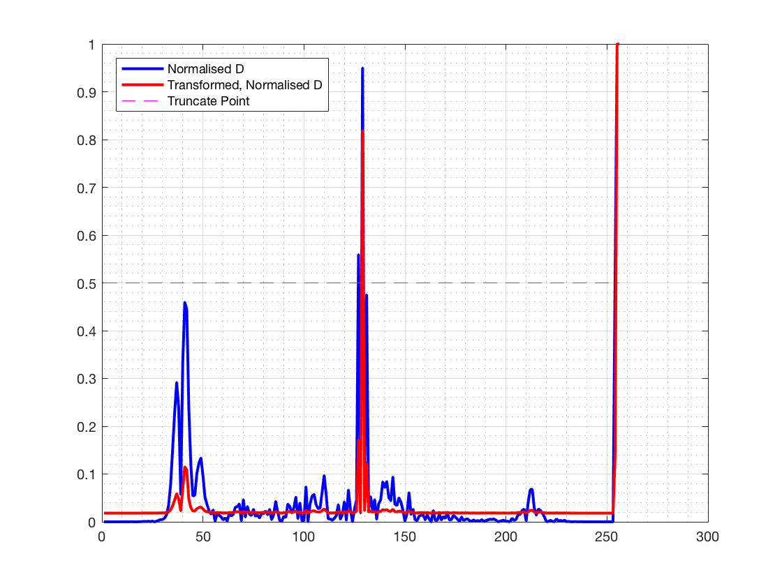
I attempted a work-around by transforming my ‘D’ by doing: $$ D’ = \exp\Bigg({\Bigg |\frac{kD}{\max{D}}}\Bigg | - k \Bigg) $$
This widened the gap between true image and monochromatic noise. I found making ‘k’ larger increased the attenuation of non-noise data, however it also attenuated other monochromatic noises present. I found k=2 to be a suitable compromise.
We can then threshold by truncating data 50% the intensity of the maximum peak. More elegant methods can be applied to detecting peaks, however I am using this method for speed and simplicity. The above is neatly summarised in a few lines of code:
function [locations] = findchroma(I,attenfact,threshold)
%FINDCHROMA Finds the locations of noise on an image's histogram, given the
%image I, an attenuation factor, and a threshold fraction.
Ihist = imhist(I);
D = abs(gradient(gradient(Ihist)));
Dp = exp(attenfact*D/(max(D))-attenfact);

locations = find(Dp>threshold);
end
N.B. We prefer gradient over diff in this situation as diff truncates the set and causes loss of peaks.
For 0.5% noise in two locations, I found the following result:
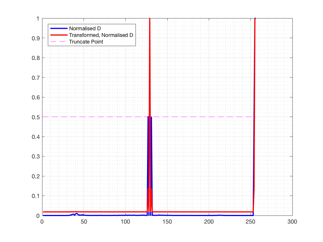
And the result I found for 15% noise in two locations:
My peak-detection worked well overall. I found higher-noise cases resulted in more accurate noise recognition.
Using the information for what colour the noise works at, we can begin by marking damaged pixels.
%Initialise the array of bad locations
Bad = false(size(I));

for i = 1:length(badvalues)
    Bad(I==badpoints(i))=1;
end
This generates a logical array with the locations where the corruption we detected earlier is present. We can now selectively apply a median to these points, as well as use some interesting properties of the histogram.
The principle of the rest of the program is to apply a ‘selective median’ on the damaged data-points, which ignores any damaged pixels to preserve all the good information we have in the image.
The improvements I’m making include:
We will end up with results better than the following…