Post

Motivation

In some electronics projects we may be required to cost-effectively generate a sinusoid. Digital systems are ubiquitous in today’s world - and powerful computational nodes such as the ESP8266 are available at extremely low prices (on the order of $1).

Generating a sine wave, however is something that can’t be done with a digital chip - usually only able to bit-bang a square wave, more expensive chips may have DACs that provide sine capability. This short post will show how to cheaply achieve a sinusoid, using passive components and a bit-banged square wave.

The Square Wave

The square wave can be decomposed through Fourier Analysis to a series of cosines or sines. More formally;

$$ f(t) = \sum^{\infty}_{k = - \infty}C_k \exp \Big (\frac{j 2 \pi k t}{T} \Big)$$ $$ C_k = \frac{1}{T} \int^{T}_{0} f(t) \exp \Big (\frac{-2 j \pi k t}{T}\Big ) \mathrm{d}t $$

We consider T to be one period of the square wave, and then know the square wave can be represented as: $$ f(t) = H(t + Tn) - H\Big(t-\frac{T}{2}n \Big) $$ Or if looking in the 0-T window.. $$f(t) = 1 - H \Big ( t - \frac{T}{2} \Big ) $$

We solve through for Ck, and find,

$$ f(t) = \frac{4}{\pi} \Big ( \cos (t) - \frac{\cos (3t)}{3} + \frac{\cos (5t)}{5} + \cdots \Big) $$

We see that our square wave is made up of a fundamental, and then all odd harmonics!

It is easy to see here that we must filter anything above the fundamental to achieve a sinusoid.

Filtering

First-Order Passive

A first-order low pass filter made of passive components looks like the following:

And has Transfer Function:

$$ G(s) = \frac{V_{out}(s)}{V_{in}(s)} = \frac{1}{1+sCR} $$

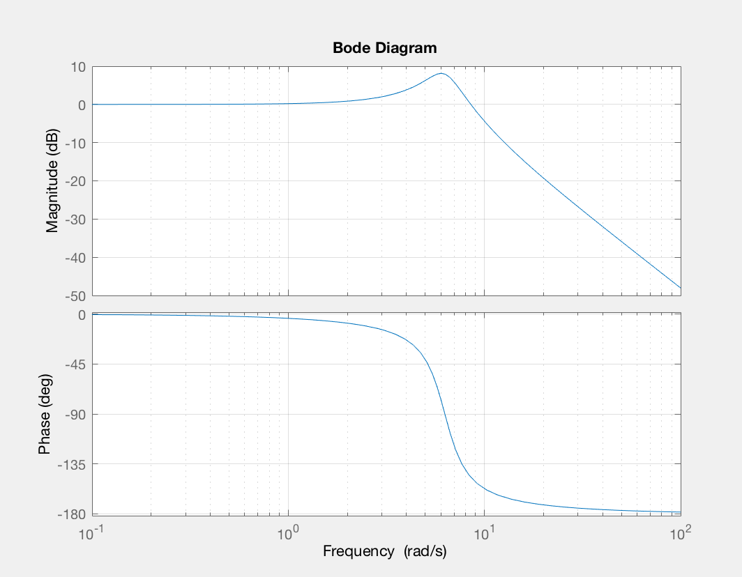
If we set $s = j\omega$ (ignoring transient behaviour - which is identical to taking the Fourier Transform) we obtain the frequency response of the filter.

If we view the Bode Plot we see we have roll-off of 20 dB per decade - which is good, but not good enough for our square wave, where we require high attenuation of the third harmonic.

We can chain two of these in a row, which is the same as doing $G^2$ for better roll-off, but we attenuate the signal by a large amount.

Second-Order Passive

Alternatively, we can consider a Second Order passive system, designed properly.

This may look like:

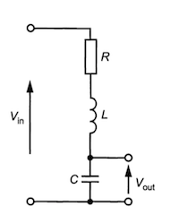
Which has Transfer Function:

$$ G(s) = \frac{V_{out}(s)}{V_{in}(s) } = \frac{1}{s^2LC + sRC + 1} $$

Comparing to a standard oscillatory system, we can note that: $$ \omega_c = \frac{1}{LC}, \qquad \zeta = \frac{R \sqrt{\frac{C}{L}}}{2} $$

So we can write:

$$ G(s) = \frac{\omega_c^2}{\omega_c^2 + 2\zeta \omega_c s + s^2} $$

Active Filtering

Active devices can be used to filter your signal. The Op-Amp is a very useful device that once was very expensive, yet now can be bought for pennies and can exist in a package 0.86mm x 0.86mm x 0.5mm. These devices can be used to make whichever filter we need - and negate the need for space-consuming inductors.

The Butterworth Filter is one such example, yet there are may other filters that can be achieved with an Op-Amp. Texas Instruments has a [very nice document] (http://www.ti.com/lit/an/sloa049b/sloa049b.pdf) that shows more filters with some component choice methods too.

Filter Simulation

I considered for this section $T = 1$, and usage of a Second-Order passive filter.

We can take the convenient form offered from the Second-Order filter section, and move to a MATLAB simulation¹ to see how our filter performs, as well as explore the effect of changing parameters.

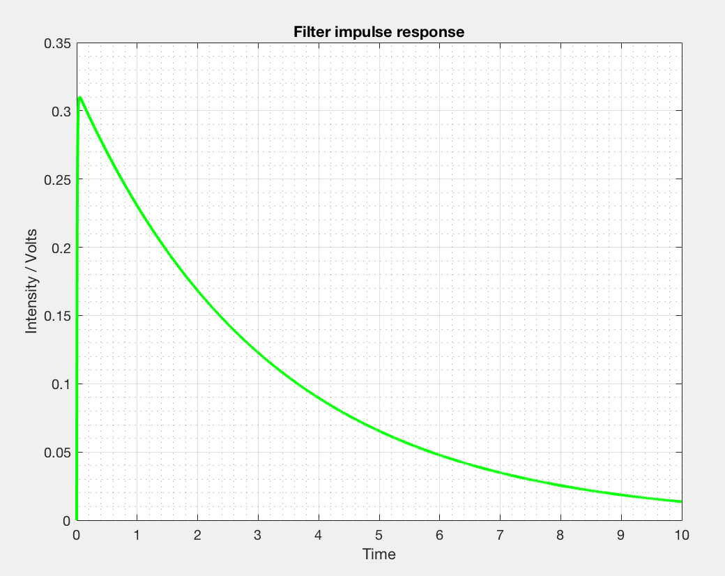
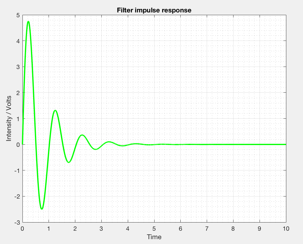
The way I considered filter application in MATLAB was to generate an impulse response from my transfer function, and then convolve with the square wave (multiplying each term by dt as this method is discrete).

We initially find that for a low damping constant, we achieve resonant behaviour, this is expected. We can place our fundamental on the resonant peak by setting $\omega_c = \frac{2 \pi} {T} $. Placing our fundamental on the resonant peak offers us a larger difference in amplitude of the fundamental and the harmonics - so I implemented that in my simulation.

The Square wave was generated using a clever trick involving the mod function, which can be quickly applied to a large array to make a Square wave.

Results

For low damping constants, we achieve amplification as well as a nice sinusoid.

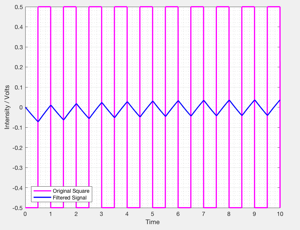
For high damping constants however, we retrieve a triangle signal. This is similar to an integrator - which makes sense as $\frac{1}{s}$ type behaviour dominates.

If we attempted a first-order filter we observe high attenuation and leakage of the first and firth harmonic into our signal - giving us a warped sine wave or a hybrid of a triangle and sine.

$\zeta = 10$ Temporal Bode Impulse

$\zeta = 0.2$ Temporal Bode Impulse

We are happy with the $\zeta = 0.2$ case, however we must recall this is with no current draw! If we want to draw current, I would suggest a voltage follower.

Done :)

That should be everything you need to extract a sinusoid!

MATLAB Simulation Code

The following MATLAB code should generate and apply your filter:

clear all; close all; clc;

s = tf('s');       %declare s as Laplace variable

%all times in seconds - freq in Hz.
tmax = 10;         %time window of simulation
dt = 0.05;         %dt of simulation
fsquare = 1;       %frequency of square wave
Amp = 1;           %amplitude (peak to peak)

wc = 2*pi*1;       %cutoff frequency of filter
zeta = 0.2 ;       %damping const. of filter

fftsize = 2^16;    %number of points the generates

%define your filter's transfer function.
G_filt = 1/( 1   +   2*zeta*s/wc   +   s^2/(wc^2) );

%make a square wave
t = linspace(0,tmax,tmax/dt);
x = 1:(tmax/dt);
k = 1/(2*dt*fsquare);
y_square = (Amp*(mod(x,2*k)- mod(x,k))/k - 0.5*Amp);

%get filter's impulse repsonse
y_impulse = impulse(G_filt,t);

%apply filter (convolve then truncate)
y_filtered = conv(y_square,y_impulse)*dt;
y_filtered = y_filtered(1:length(y_square));

%plot bode response of filter
figure();
bode(G_filt);
grid; grid minor;

%plot impulse response of filter
figure();
plot(t,y_impulse,'g','linewidth',2);
title('Filter impulse response')
xlabel('Time')
ylabel('Intensity / Volts')
grid; grid minor;

%plot original signal
figure();
plot(t,y_square,'m','linewidth',2);
xlabel('Time')
ylabel('Intensity / Volts')
hold on

%plot filtered response
plot(t,y_filtered,'b','linewidth',2);
xlabel('Time')
ylabel('Intensity / Volts')
grid; grid minor;
legend('Original Square','Filtered Signal','Location','southwest')

%make user pick point at which transients are gone
uiwait(msgbox('Pick the point on the graph where the transients are gone.'));
[t_truncate,~] = ginput(1);
n_truncate = round(t_truncate/dt);

%truncate the filtered dataset and shift to zero to remove DC component.
y_filtered_truncated = y_filtered(n_truncate:end);
t_truncated = t(n_truncate:end);
y_dc = trapz(y_filtered_truncated,t_truncated)/(t_truncated(end) - t_truncated(1));

%run ffts
Y_fil = fft(y_filtered_truncated,fftsize);
Y_sq = fft(y_square(n_truncate:end),fftsize);

%evaluate power spectra
Pyy_sq = Y_sq.*conj(Y_sq)/fftsize;
Pyy_fil = Y_fil.*conj(Y_fil)/fftsize;
freq = (1/dt)*(0:(fftsize/2))/fftsize;

%plot fft for square
figure();
plot(freq,Pyy_sq(1:(1+fftsize/2)),'k','LineWidth', 2);
xlabel('Frequency (Hz)');
ylabel('Power');
hold on

%plot fft for filtered data
plot(freq,Pyy_fil(1:(1+fftsize/2)),'r','LineWidth', 2);
title('Signal FFTs')
xlabel('Frequency (Hz)');
ylabel('Power');
grid; grid minor;
legend('Square Wave','Filtered Signal','Location','northeast')