Post

The what?

There comes a time in every computer-oriented blog where this post is made, rather than delaying the inevitable, I feel it is time to commit to writing and get it over with.

This post is about one of the best approximations of all time, the Fast Inverse Square Root.

I’d like to go over why we need this first, since I rarely have encountered detailed backgrounds.

Normal Vectors

In computer graphics, normalised vectors ($L_2$ magnitude of the vector is 1, or more formally $||\hat{\mathbf{v}}||_2 = 1$) are used a lot for lighting (luminence, shadows, reflections and more).

By a lot, I mean millions of times a second, as every angle of incidence and reflection is calculated using these vectors, $\hat{\mathbf{v}}$.

Before I discuss why this is such a problem, I would first like to discuss how we get these vectors ($\hat{\mathbf{v}}$).

Objects in computer graphics are polygons defined as a set of surfaces, which have 3D coordinates $\mathbf{x}_i = (x_i,y_i,z_i)$ for each vertex (corner). Triangles are commonly used as they have three vertices, the minimum number required to define a flat plane.

Using the set of three points used to define the surface $ \mathbf{x}_1, \mathbf{x}_2, \mathbf{x}_3 $ we can now try and find a surface normal.

We can consider $\mathbf{x}_1$ as our reference point for the object, and define the order of the points (1,2,3) to be what we would see if we look face on and proceed anti-clockwise around the polygon. The anti-clockwise property is important and I shall explain later.

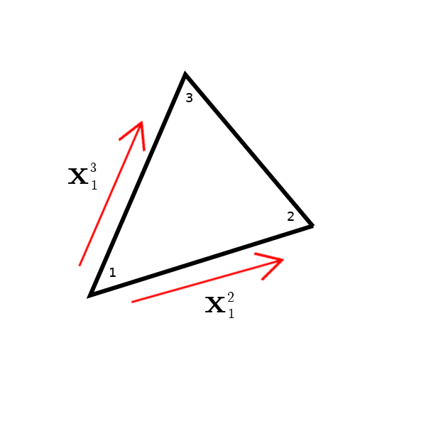
To further set up the problem, we now need to find the difference between our other vertices and the reference point as the vector from $\mathbf{x}_1$ to $\mathbf{x}_i$ where $i$ is 2 or 3. I am going to use the shorthand $\mathbf{x}_1^2 = \mathbf{x}_2 - \mathbf{x}_1 = (x_2-x_1,y_2-y_1,z_2-z_1)$ to resemble this vector.

It might be easier to show diagrammatically, before we make any further steps. The diagram below shows a triangle we are looking at that is facing us (surfaced side up).

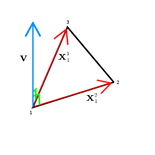
From here it is relatively easy to get the normal! We have an oriented surface now defined by two vectors, so we can take the cross product ($\mathbf{x}_1^2 \times \mathbf{x}_1^3 = \mathbf{v}$).

A cross product is an operation that exists only in three and seven dimensional spaces which allows us to multiply two vectors in such a way that a new vector is made which is orthogonal (at right angles) to both of the two generating vectors.

The benefit of the way we oriented our triangle is that the surface normal will be emerging from the side which has the top of the surface.

A diagram is provided to aid understanding on what we have just done:

To humour ourselves, although not the goal of this post, we can test for polygon visibility. We have $\mathbf{v}$, we can run a simple test to see if the polygon is facing us. If we draw a vector from the surface to the location of the observer and call it $\mathbf{w}$, we can take the dot product, and if $\mathbf{w} \cdot \mathbf{v} > 0$, the surface is facing us.

Normalised Normals

As I mentioned at the beginning of this post, we are interested in normalised surface normals, which I named $\hat{\mathbf{v}}$.

There is fortunately a method to calculate this, we take the Euclidean Norm (which is Pythagoras’ theorem in higher dimensions - try it, the proof is simple) and divide $\mathbf{v}$ by it.

$$ \frac{\mathbf{v}}{||\mathbf{v}||_2} = \hat{\mathbf{v}}, \qquad \text{such that} \quad ||\hat{\mathbf{v}}||_2 = 1$$

Where $$ \mathbf{v} = (x_v,y_v,z_v) \qquad ||\mathbf{v} ||_2 = \sqrt{x_v^2 + y_v^2 + z_v^2}$$

so in one equation we can get our $\hat{\mathbf{v}}$: $$ \hat{\mathbf{v}} = \frac{(x_v,y_v,z_v)}{\sqrt{x_v^2 + y_v^2 + z_v^2}}$$

Let’s program it in our computer from the 1990s and give it a burl! Wait, why is everything so sluggish?

It turns out that floating point division and square roots are really slow for computers before efficient versions of those methods existed on-chip. Multiplication is fast, addition and subtraction are fast, but division and square roots are recursively defined and are very slow.

All of our problem used multiplication, subtraction and addition up until the point where we needed to normalise.

This begs the question, is there a way to rephrase it as problem of multiplication, so we can run this millions of times a second?

If we allow ourselves to imagine we have an algorithm that finds $a = \frac{1}{\sqrt{b}}$, then we can do $\hat{\mathbf{v}} = a (x_v,y_v,z_v)$. This is just multiplication which should be fast! All we need is the impossible algorithm that finds $a$ in a timely manner.

The good bit

John Carmack was the lead programmer of Wolfenstein 3D, Doom, Quake, Rage and Commander Keen, so it is fair to say he knows a lot about computer graphics. He was one of the pioneers of computer graphics in the 1990s, and he wrote that magical algorithm which performs a fast inverse square root.

What lies ahead is madness, so buckle up and don’t be worried if it makes no sense.

float Q_rsqrt( float number )
{
	long i;
	float x2, y;
	const float threehalfs = 1.5F;

	x2 = number * 0.5F;
	y  = number;
	i  = * ( long * ) &y;                       // evil floating point bit level hacking
	i  = 0x5f3759df - ( i >> 1 );               // what the fuck? 
	y  = * ( float * ) &i;
	y  = y * ( threehalfs - ( x2 * y * y ) );   // 1st iteration
//	y  = y * ( threehalfs - ( x2 * y * y ) );   // 2nd iteration, this can be removed

	return y;
}

Although we were probably most fixated on the humorous (original) comments, we have a lot of complicated ideas going on in one place, so let’s break it down and see if we can figure out how it works.

We have a function which takes a float number and returns a float. This is fine.

We start by defining some variables and a constant. We have a long integer i, two floats x2, y and a constant float threehalfs. This, also, is fine.

We then set x2 = number * 0.5F and y = number, if you are unfamiliar with C, we can define a float by putting an F at the end of a number. Again this is fine.

Suddenly it’s anything but fine. We are presented with:

	i  = * ( long * ) &y;                       // evil floating point bit level hacking

We know we are always passing positive values into Q_rsqrt by nature of this problem, so the sign bit will be zero! All we have to worry about is the exponent and mantissa, which I will interpret as integers and label them $E$ and $M$.

32 bit floats use the mantissa and exponent (ignoring sign) to define numbers as follows:

$$ n_{\text{float}} = \Big (1+ \frac{M}{2^{23}} \Big) 2^{E-127}$$

If we directly interpret the float as an integer, we have:

$$ n_{\text{int}} = M + 2^{23}E $$

Now we have the background covered, let’s dive into the hack behind this line of code.

We begin by taking the logarithm of $n_{\text{float}}$.

$$ \log_2 ({n_f}) = \log _2 \Big (\Big (1+ \frac{M}{2^{23}} \Big) 2^{E-127}\Big)$$ $$ \log_2 ({n_f}) = \log _2 \Big (1+ \frac{M}{2^{23}} \Big) + {E-127}$$

If we squint hard enough (and boy do you have to squint), it looks similar the integer representation although out by a constant and a multiplicative coefficient!

This is due to the fact we can approximate $\log_2(1+x) \approx x$ for $ x < 1$. We are then left with:

$$ \log_2 ({n_f}) \approx \frac{M}{2^{23}} + {E-127}$$

Giving us:

$$ \log_2 ({n_f}) \approx 2^{23}n_i + C $$

For some constant $C$.

It’s a bit of a jump, but we can say interpreting a float as an int is a poor-man’s logarithm with base two! Hummus and Magnets does a much better job of explaining this, and the interested reader is guided there to see the full derivation.

It’s good to review what we now have at our disposal, we have taken a number $b$, and we now have basically (in integer form) $\log_2(b) + K$ where $K$ is some error constant from the conversion.

	i  = 0x5f3759df - ( i >> 1 );               // what the fuck? 

This line tells us a lot, so let’s break it down.

( i >> 1 ) Tells us we are right shifting the integer i by one place. This is actually an integer division by two. So what do we have now?

$$ \frac{K}{2} + \frac{1}{2}\log_2(b) $$

But we are subtracting this, the code does say after all - (i >> 1), what do we have?

$$ - \frac{K}{2} - \frac{1}{2}\log_2(b) = - \frac{K}{2} + \log_2 \Big(\frac{1}{\sqrt{b}} \Big) $$

By Jove! Do see that? Is that an inverse square root?

Let’s put this line together, we are clearly onto something. I think you can probably see where $\frac{K}{2}$ comes in to put this together, yes, I’m talking about 0x5f3759df.

So altogether we have found the logarithm of the inverse square root of $b$ as an integer.

How do we get our float back and remove that pesky logarithm?

	y  = * ( float * ) &i;

Fantastic, we just pull the inverse of same scam we did earlier. This would also introduce an error constant but I am assuming we took care of it in the previous step.

Since this is the inverse of the original hack we used, it is a poor-man’s un-logarithm. This step also conveniantly fixes our scaling problem of $2^{23}$ which we encountered above.

	y  = y * ( threehalfs - ( x2 * y * y ) );   // 1st iteration
//	y  = y * ( threehalfs - ( x2 * y * y ) );   // 2nd iteration, this can be removed

	return y;

Now we are taking our victory lap around this function, what you see above is Newton’s method, which is an iterative equation that allows you to solve equations with linear approximations. It’s run once here just to gain a fair headroom of extra accuracy, since the rest of the function was very sketchy.

And then we just return our float!

This function is so damn fast, it actually beats lookup tables in terms of speed on the order of five times, a very significant speed increase.

Considering the sheer number of times an inverse square root is needed in computer graphics, it makes sense to go to these extremes.

And there you have it! I promised you the best approximation of all time, and I firmly believe this is it, or at least the most computed one.

You can now think to yourself when you fire up the original Quake “I know why this is fast”.