Post

Current Status

This work is currently available to everybody via the SimSPAD GitHub page.

Motivation

My DPhil research’s thrust was using silicon photomultipliers (SiPMs) as recievers to achieve optical wireless data links. SiPMs are very interesting devices, as they have the ability to detect individual photons, which means they can operate links at extremely low optical powers. The number of detected photons per bit is so remarkably low, that the system is limited by Poisson statistics.

This combined with the fact that the SiPM has a large active area, high detection efficiency, and high bandwidth makes them an ideal candidate for being receivers for optical wireless communications.

What is a SiPM?

A SiPM is a device which has a large array of avalanche detectors, called microcells. The majority of devices which can be purchased are passively quenched, which means that a resistor is used to halt the avalanche process, and allow the microcell to recharge. This small but fininte (tens of nanoseconds) recharge time causes nonlinearity in the electrical response.

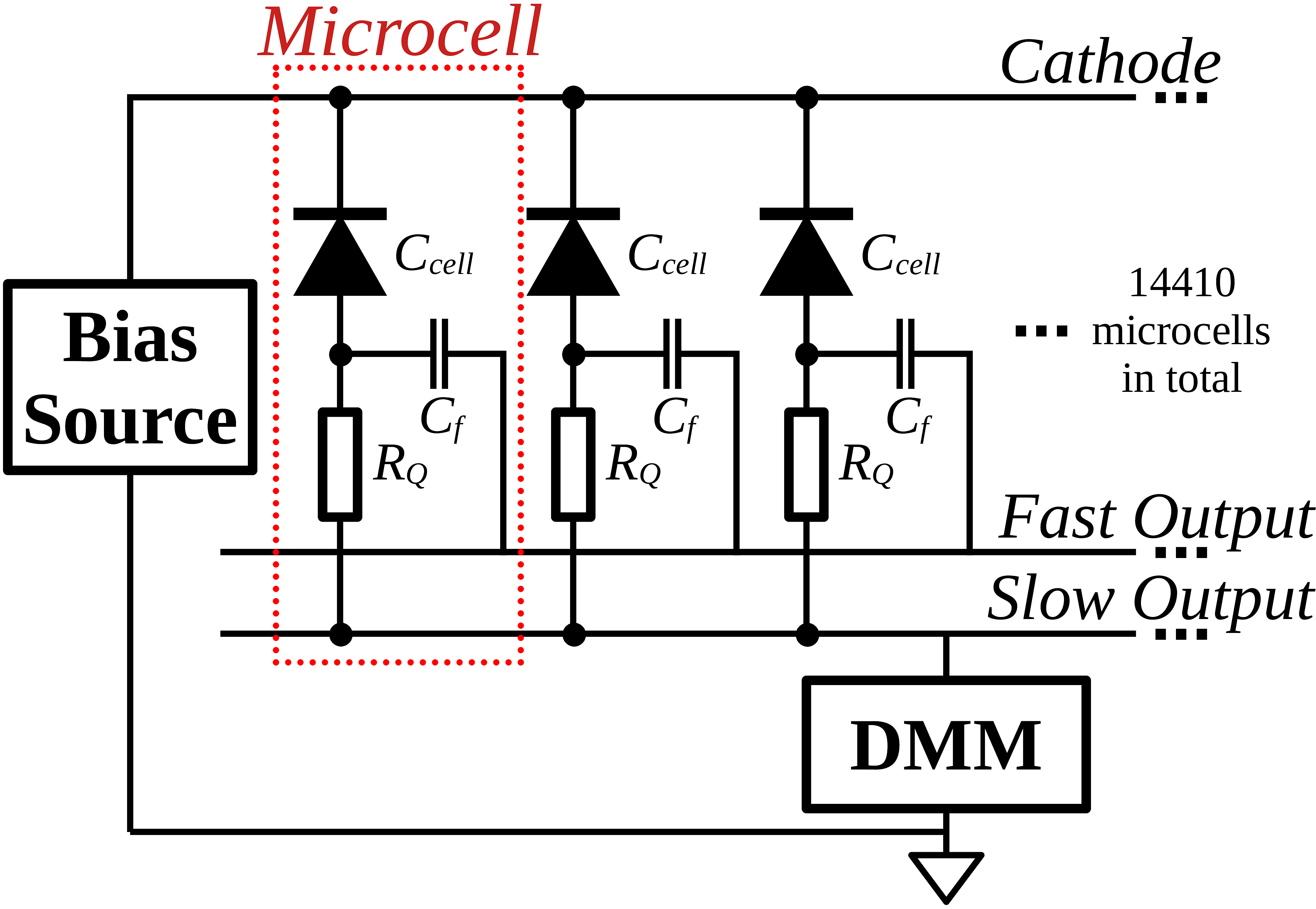
With SiPMs, the output is often taken in series by measuring the bias current emittedby the device. Unfortunately, this output is exceptionally low bandwidth, as the output is limited by the RC recovery time constant of the recharging process. Instead, some manufacturers like Onsemi produce devices which have a ‘fast output’. This high-bandwidth output is coupled to each of the avalanche diodes, and gives the user a common high bandwidth line, where each of the detection pulses are visible with a 1.5ns full width half max time. Given the current state of research, I believe that the future of these devices will be using fast outputs fed into signal processing silicon.

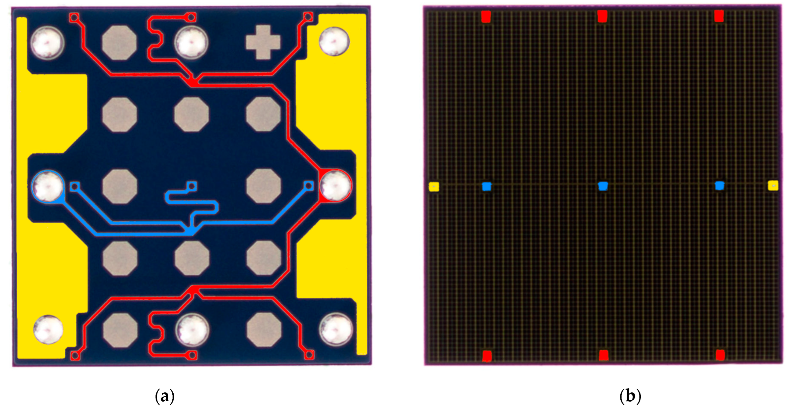
This image shows a view of a J series 30035 SiPM from Onsemi. (a) shows the back of the SiPM, where different traces are highlighted different colors for visibility. Yellow is the cathode (connected to bias source), blue is the anode (connected to ground, or a series resistor to measure instantanous bias current). Red traces are the fast outputs. The fast output on this device is combined from six separate regions. (b) shows the top of the SiPM, where the through-silicon via processes connect to the traces on the rear.

Electrically, this SiPM (and other passively quenched SiPMs with a fast output) appear as the following:

Microcell Recharging

After a photon has been detected by a microcell, that microcell must recharge. This can be simply modelled by assuming the device is a capacitor¹

$V_{\mu}(t) = V_{\text{over}} \left(1 - \exp \left(-\frac{t}{\tau_{rc}}\right) \right) $

Where $\tau_{rc}$ is the RC time constant for the microcell recharge rate, and $V_{\text{over}}$ is the overvoltage applied to the SiPM ($V_{\text{bias}} - V_{\text{breakdown}}$).

From some of my earlier work, I was able to create a model for the photon detection efficiency $\eta$ of onsemi SiPMs:

$\eta(V_{\mu}) = \eta_{\max} \left ( 1 - \exp \left ( \frac{-V_{\mu}}{V_{\text{chr}}} \right) \right) $

Where $\eta_{\max}$ is a parameter dictating the maximum PDE at infinite overvoltage and $V_{\text{chr}}$ is a characteristic voltage for the avalanche diode.

How Detection Works

When a photon strikes a microcell, it has a probability it will cause an avalanche. This probability is in fact the product of other random processes.

1. When a photon strikes the PN junction there is a probability that it will create an electron-hole pair.
2. There is then a probability that the electron will reach the depletion region where the high voltage gradient can lead to avalanche multiplication. This may not happen as the electron randomly walks and may recombine with a hole in the silicon.

Point two is especially interesting as the time since the last detection changes the voltage and hence the depletion region width.

Nonetheless, the probability of detection given a photon has struck the microcell is encapsulated in $\eta(t)$.

Given that a microcell avalanches, the output charge will be however much charge has built up in the capacitance of the PN junction.

By using the capacitor analogy from ealier, this charge $Q_{\mu}$ can be found from our friendly old $Q=CV$. $$ Q_{\mu}(t) = C_{\mu}V_{\mu}(t) $$

Interestingly, the microcell can detect a photon while it is recharging². This doesn’t even seem to be an unreasonable assumption, as it’s similar to the microcell detecting the photon with a different overvoltage and hence PDE and charge.

A Statistical Observation

Photon arrivals at the detector are exponentially distributed in time. $$ f_{\gamma}(t;\lambda) = \lambda \mathrm{e}^{-\lambda t} $$ However the fact that microcells must recharge after detection, and that immediately post-detection $\eta = 0$ means that the pdf of the the microcell interdetection time must have a boundary condition at zero time $f(0;\lambda)=0$. Finally as the PDF is continuous and smooth, this means we need a radically different probability function.

As we mentioned before, the photon detection efficiency depends on the microcell overvoltage, which further depends on the time since last detection. This can be used to create our new distribution, which is something called a renewal process. $\eta(t)$ modifies the shape of exponentially distributed interphoton arrival times to form a new distribrution of the interdetection times.

$$ f_{\mu}(t;\lambda) = \eta(V_{\mu}(t)) \lambda \mathrm{e}^{(-\lambda t p_{\mu}(t))} $$

where

$$ p_{\mu}(t) = \frac{1}{t} \int_0^t \eta(V_{\mu}(t)) dt $$

While useful, this distribution does not help us if we wish to equalise the output, as it only tells us the distribution of interdetection times.

For an arbitrary stopping time at constant irradiance, the probability density function can be shown to be:

$$ f_x(t) = \frac {\int_t^{\infty} f_t(t) dt} {\int_0^{\infty} \int_t^{\infty} f_t(t) dt dt} $$

Microcell Initialisation

Before simulation can begin, the microcells must be initialised with randomly distributed times since detections. We can use the previous derivation to our advantage, as we can now construct a probability distribution function and simply draw random samples from it.

Unfortunately, we cannot make a fully accurate prediction of the history of the incident photons, as we have no knowledge of the past before the simulation begins. Instead, we use a simple approximation where the mean number of expected photons throughout the simulation is used as the assumed past. This is a reasonable approximation, as this places the SiPM in a state reasonably close to what it would be if the previous incident light was simulated.

Simulation

To simulate the device, we use a simple Monte Carlo method. The simulation takes a vector of the number of expected incident photons per time step. For each time step, a Poisson random variable is drawn where the mean is the number of expected photons. This Poisson random variable is the number of photons which are now incident on the device. For each of these photons, a uniform random distribution is used to select a microcell.

The selected microcell’s photon detection is then simulated. Each microcell has an internal state which is the time since last detection. This time is calculated using the microcell’s time when a photon was last detected, and the current simulation time. The time since last detection determines the microcell’s overvoltage, which is used to calculate the photon detection efficiency.

Calculating the overvoltage and photon detection efficiency is a computationally expensive process, as it requires exponentiation and division. To speed up the simulation, the overvoltage and photon detection efficiency are precalculated for a range of times since last detection. These values are stored in a lookup table, and the simulation uses linear interpolation to find the correct value for the current time since last detection.

The photon detection efficiency is used to determine if the microcell detects the photon. A random sample from a uniform distribution is drawn, and if the sample is less than the photon detection efficiency, the microcell is said to have detected the photon. If the microcell detects the photon, the microcell’s last detection time is updated, and the microcell’s output charge is calculated. The output charge is then added to the microcell’s output charge buffer, which is used to determine the fast output for a single time step.

Two flowcharts are shown below, which show the simulation process for a single time step, and the simulation process for a single photon detection.

The Road Towards Optimal Equalisation

So far, we have only discussed the simulation of a SiPM, and not the equalisation of the output. The equalisation of the output is a difficult problem, as the output is a function of the microcell’s output charge, which is a function of the microcell’s overvoltage, which is a function of the time since last detection, which depends on the history of incident light.

The first step towards equalisation is to determine the probability density function of the time since last detection for an arbitrary stopping time and history of incident light. This is a difficult problem, as the probability density function is a function of the history of incident light, which is a function of the probability density function. This is a chicken and egg problem, and so far I have not been able to find a solution, but I have found a reasonable approximation in a numerical solution, backed up by some analytical results.

My numerical solution outputs the expected output charge, and a probability density function of the time since last detection for each time step. Both of these outputs depend on the history of incident light.

This is achieved by simulating the PDF and evolving it over time. The simulation begins with an initial guess of the probability density function, $P(x,t)$, where $x$ is the time since last detection, and $t$ is the current simulation time. In a steady state, the PDF does not change with time and so $P(x,t+dt) = P(x,t)$. The detection probability for each $x$ is $\eta(x)$.

The PDF can be evolved over time using using the following process: $$ P’(x,t+dt) = P(x,t) \left ( 1 - dt \lambda \eta(x) \right) $$ Where $\lambda$ is the mean number of photons per time step. $P’$ lacks the initial element for $x=0$, and so the following equation is used to update the probability density function: $$P(x+dt,t+dt) = P’(x,t+dt) $$ $$P(0,t+dt) = \sum_{x=0}^{\infty} P(x,t) dt \lambda \eta(x)$$

What this process does is:

1. The probability density function is updated using the previous probability density function, and the probability of detection for each $x$.
2. The probability density function is shifted in time by one time step.
3. The probability density function is updated for $x=0$. The density at $x=0$ encapsulates the microcells which have detected a photon in the current time step.

This process is repeated for each time step, and the evolution of the probability density function can be observed. The expected output charge is one of the outputs of this process, but what is more interesting is the probability density function of the time since last detection. This probability density function can be used to equalise the output of the SiPM.

The PDF can be used to calculate the expected photon detection efficiency and the gain of the SiPM at each time step. Dividing the actual output charge by the expected output charge gives the equalised output charge. This equalised output may be used in a receiver to increase a link’s SNR.

When equalising the output, the incident photon rate must be known for each time step. As the incident photon rate is not known, the incident photon rate is estimated using previous equalised output. This might be a bad idea, and I am currently investigating other methods of estimating the incident photon rate. The problem feels similar to DFE, and I suspect that a similar solution may be possible.

A toy example of this process is available in the code block below.

Thoughts and the future

I have been able to simulate the SiPM, and (I think) I have been able to equalise the output. This may be a good starting point for a paper on equalisation of SiPMs, and I think this research is worth pursuing further.

The simulation, as it stands, is very fast. Its implementation is freely available on GitHub, and I would be keen to see if others can use it to achieve similar results. I plan on updating the server API to use RPC, as the current implementation is a bit of a hack (a big vector of doubles is sent over HTTP, encoded as characters).

If you have any questions, please feel free to contact me, or open an issue on GitHub. I would be happy to discuss this work further, and collaborate with others on equalisation of SiPMs.

import numpy as np
import matplotlib.pyplot as plt


vover   = 3.0
taurc   = 2.2 * 14E-9
ccell   = 14E-15
pdemax  = 0.46
vchr    = 2.04


def vcell(t):
    return vover * (1-np.exp(-t/taurc))

def qcell(t):
    return vcell(t) * ccell

def pde(t):
    return pdemax * (1-np.exp(-vcell(t)/vchr))

def evolve_PDF(P, lam):
    global pdes
    global charges
    # for steady state
    #P(x,t+dt) = P(x,t)

    Pdiff = P*dt*lam*pdes
    P = P-Pdiff
    #P(x,t+dt) = P(x,t) * (1 - dt * lam * pde(x))

    end = P[-1] # cut off end
    P = np.delete(P,-1)
    P[-1] += end # don't lose prob mass
    P = np.insert(P, 0, np.sum(Pdiff)) # shift in time
    qfired = np.sum(Pdiff * charges)
    return (P, qfired)

def calc_dist_params(P):
    global pdes
    global charges
    #global ts
    #plt.plot(ts, pdes*charges)
    #plt.plot(ts, P*pdes*charges)
    lambda_est = np.sum(P*pdes*charges)
    return lambda_est

# Time step and Max Time for PDF
dt    = 1E-10
tmax  = 50E-9

# Times for the PDF, PDEs for each time, and Qcell for each time
ts = np.array([i*dt for i in range(int(tmax/dt))], dtype=np.float64)
pdes = pde(ts)
charges = qcell(ts)

# Create PDF array and set initial state (All microcells have zero charge)
P0 = np.array([0.0 for _ in ts], dtype=np.float64)
P0[0] = 1.0/dt
Pe = P0.copy()

# Simulation Params
doonoff = True              # Do we do ook?
onoff_period = 1E-9         # Bit Time
high_level = 1.8E9          # Bit One level
low_level  = 1.8E8          # Bit Zero Level
clock = 0                   # Vary clock to change phase

# Let the number of iterations needed be twice the length of the PDF
numsamp = len(ts)*2

# Output Fired Charge, and output Time Array Init
qfired = np.array([], dtype=np.float64)
qfired_eq = np.array([], dtype=np.float64)
times = np.array([], dtype=np.float64)

# Init simulation parameters - users should not change these
bit = 1                     # Starting bit level
time = 0                    # Simulation start time
arrivalRate = high_level    # Starting photon arrival rate

print("Running", numsamp, "Iterations...")
for i in range(numsamp):

    # On-off demonstration block
    if (clock > onoff_period) and doonoff:
        clock = 0
        # bit = not(bit)
        # if bit:
        #     arrivalRate = high_level
        # else:
        #     arrivalRate = low_level
    arrivalRate = (high_level*clock)/onoff_period

    # Update the PDF
    Pe, qf = evolve_PDF(Pe, arrivalRate)

    # Store fired charge, time and increment the time
    qfired = np.append(qfired, qf)
    qf /= calc_dist_params(Pe)
    qfired_eq = np.append(qfired_eq, qf)
    times = np.append(times, time)
    time += dt
    clock += dt

# Print accumulated error
print(100*(np.sum(P0) - np.sum(Pe))/np.sum(P0), "% Error in distribution mass")

# Kill final element in PDF - as this stores \int_tmax^\infty P(t) dt
Pe[-1] = Pe[-2]

# Plot PDF
plt.figure()
plt.plot(ts, Pe)
plt.xlabel("Time Since Last Detection [s]")
plt.ylabel("Prob Density")

# Plot Log PDF
plt.figure()
plt.plot(ts, np.log(Pe))
plt.xlabel("Time Since Last Detection [s]")
plt.ylabel("Log Prob Density")

# Plot EXPECTATION of response
fig, ax1 = plt.subplots()
ax1.plot(times, qfired)

ax2 = ax1.twinx()
ax2.plot(times, qfired_eq, 'C1')
ax1.set_xlabel("Time [s]")
ax1.set_ylabel("Expectation of SiPM Response $E[y(t)]$")
ax2.set_ylabel("'Equalised'Expectation of SiPM Response $E[y(t)]$")

plt.show()