Post

Wait, this isn’t a post on Ray Tracing?

Well not quite, I don’t mean “ray tracing” in the sense of scene rendering in computer graphics. My research is based on some very specific optical devices and I am interested in how geometry impacts their performance.

Ray tracing is typically complicated, but ‘Ray Marching’ is a simplified way to achieve a very similar result.

What I’m interested in “ray tracing” is the optical path a single ray will take inside the device - so by running Monte-Carlo simulations I can estimate the statistical nature of the device (exit angle, exit location, optical path length and more).

A two-dimensional example of what is expected to be achieved is shown here:

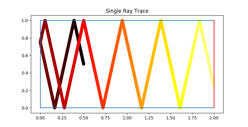
We can also move into the third dimensional realm, but it is only a small extension on the logic presented in this post.

Some notes on Rays

Representation

A ray in a fundamental sense is a tuple of two vectors, a ray will have a position and a direction associated with it all the time it is active. Expressing a ray as a pair of two vectors is extremely useful as it allows for efficient reflection and propagation formulae to be written. We also have operations like normalisation when vectors are used - much to our benefit.

In a Python implementation of this program, I use the dictionary object (for nice mutable properties) to create a ray object:

rayObj = {"dir": [1,0], "pos": [0,0]}

Which for this case is a ray located at the origin which will move in the positive x direction.

Propagation

As we are using an arbitrary geometry for our ray tracer to reflect inside, I decided to use an Euler step by step method rather than setup any fancy linear equations to solve (and slowly lose my mind over when it doesn’t work). I define a step length $\mathrm{d}l$ which allows our ray to move with each simulation iteration:

rayObj["pos"] += rayObj["dir"] * dl

The direction of the ray does not change when propagating (if the refractive index is constant), but it does when reflecting off a surface…

Reflection

A ray will reflect (specularly) when it hits a specular surface. Surfaces are conveniently defined to have a surface normal, which is a vector pointing perpendicularly to the surface.

On contact with a surface, a ray reflection can be efficiently represented by the following vector operation:

def reflect(rayObj):
    rayObj["dir"] += - 2 * np.dot(rayObj["dir"], surf_norm)
    rayObj["dir"] = normalise(rayObj["dir"])

With np of course being numpy. The position of the ray does not change when reflecting.

Normalisation

Normalising vectors is a really handy tool to have in your belt - so I define it quickly here for convenience.

def normalise(x):
    return x / np.linalg.norm(x)

Let’s define our Stage

For ease of use and the sake of my rapidly deteriorating sanity, I use the Python Shapely package to define the polygon used to define the “simulation stage”.

This of course requires some imports:

from shapely.geometry import Point, LineString
from shapely.geometry.polygon import Polygon

Using Shapely it is extremely quick to move from a set of coordinate points to a polygon as noted below. While here - I also define what type of edge will be used - whether it will reflect rays (mirror “m”) or absorb and detect them (detector “d”).

nodes = [[0,0],[0,1],[2,1],[2,0]]                                                        
edge_types = ["m", "m", "d", "m"]
poly = Polygon([n for n in nodes])

Now it gets a little tricky - we need to package this up into a convenient form for the ray tracer to use (and also find those surface normals!). Again we can use a dictionary object - its nice mutable properties may come in handily later. We start with saving the polygon, and the range in the x and y axes where the stage exists.

stage = {"polygon":poly,
    "edges":{},
    "xrange": [min([x[0] for x in nodes]),max([x[0] for x in nodes])],
    "yrange": [min([x[1] for x in nodes]),max([x[1] for x in nodes])]
    }

Note that we created a ’edges’ dictionary, despite having a Shapely polygon defined. We can define the edges as lines (Shapely LineStrings), which will come in use later. The most important process in this step is finding the surface normal (saved as “dir” - the direction of the surface) which is a relatively simple ordeal:

for i in range(len(nodes)):
    edge1 = nodes[i]
    if i == len(nodes)-1:
        edge2 = nodes[0]
    else:
        edge2 = nodes[i+1]

    dx, dy = edge2[0] - edge1[0], edge2[1] - edge1[1]
    if edge_types[i] == "m":
        t = "mirror"
    elif edge_types[i] == "dump":
        t = "dump"
    elif edge_types[i] == "d":
        t = "detector"
    else:
        raise ValueError("Undefined or Incorrectly defined edge type: " + str(edge_types[i]))
    print(edge1, edge2)
    stage["edges"][i] = {"from":edge1, "to": edge2, "dir":np.array([dy,-dx]) , "line": LineString([edge1, edge2]) ,"type":t}

Great, now can we ray trace?

Simulating rays interacting with the Stage

We can now work on a function sim_ray which will return an optical path.

First let’s define some requirements of this function.

1. It must be able to reflect a ray on contact with a surface
2. It must be able to terminate if a ray reflects forever
3. It must accurately be able to know when to terminate - has it struck a detector?
4. It must be able to return an optical path length of the ray
5. It must be able to return an optical path of the ray
6. It must be able to accurately determine if a ray has struck a surface (or edge in this 2D case)

To put it all down in one go, the solution looks like this:

def sim_ray(ray, stage, dl=0.1):
    detected = False
    itercount = 0
    path = []
    while not detected:
        if itercount > 10000:
            return None, None
        itercount += 1
        oldray = copy.deepcopy(ray)
        path.append(oldray["pos"])
        ray["pos"] += ray["dir"] * dl
        if not stage["polygon"].contains(Point(ray["pos"][0], ray["pos"][1])):
            ## find intersecting line...
            test_line = LineString([(ray["pos"][0], ray["pos"][1]), (oldray["pos"][0], oldray["pos"][1])])
            for e in stage["edges"].keys():
                intersection = (stage["edges"][e]["line"].intersection(test_line))
                if not intersection.is_empty:
                    do_reflect, ref = (True if stage["edges"][e]["type"] == "mirror" else False), e
                    is_dump = (True if stage["edges"][e]["type"] == "dump" else False)
                    break
            else:
                print("NO INTERSECTION ERROR")
                return None, None

            if do_reflect:
                ray["pos"] -= ray["dir"] * dl
                wall = normalise(stage["edges"][ref]["dir"])
                ray["dir"] = reflect(ray, wall)
            else:
                if is_dump:
                    return None, None
                return path, itercount * dl

A lot is going on here so let’s break it down and discuss each part.

The while not detected is pretty self explanatory, as well as the following two lines on terminating if the ray is taking an extremely long time to reach the detector.

The first thing you may raise a question with is the oldray = copy.deepcopy(ray). This is due to the mutability of the dictionary type - doing oldray = ray means the two objects are directly related and editing one means editing the other. As we are storing the old ray - we need to duplicate in a safe way with a deepcopy.

After that we encounter our earlier defined ray propagation equation: ray["pos"] += ray["dir"] * dl which isn’t a surprise, but what follows may be.

We are faced with the expression if not stage["polygon"].contains(Point(ray["pos"][0], ray["pos"][1])): What this basically says is “if the ray’s position is not inside the polygon we defined earlier as our stage - do something”. This was the primary reason for picking Shapely - we can very quickly work with edges in this manner, and its existence saves a lot of our time.

What the “do something” actually is follows in the indented block. We know that we had to pass through an edge from our last iteration to this iteration, so we can now identify it. We first construct a line between the last iteration’s position and the current iteration’s position as test_line.

Now that we have our line to test against, we can test each edge in our polygon to see if it intersects our line (another wonderful piece of functionality that shapely offers):

for e in stage["edges"].keys():
    intersection = (stage["edges"][e]["line"].intersection(test_line))
    if not intersection.is_empty:
        do_reflect, ref = (True if stage["edges"][e]["type"] == "mirror" else False), e
        is_dump = (True if stage["edges"][e]["type"] == "dump" else False)
        break

We also store some flag variables like do_reflect, is_dump as well as an edge reference ref for use in the following few lines:

if do_reflect:
    ray["pos"] -= ray["dir"] * dl
    wall = normalise(stage["edges"][ref]["dir"])
    ray["dir"] = reflect(ray, wall)
else:
    if is_dump:
        return None, None
    return path, itercount * dl

This small section of the code is responsible for the reflection and termination!

If the surface is reflective, the ray’s position is backed out by a single iteration for safety (although this should be placed at the intersection point - something that has changed since this version). After the position has been backed out - the wall’s surface normal is obtained and the reflection is performed.

If the surface isn’t reflective, and the surface isn’t a “beam dump” (so therefore must be a detector), the path and optical path length are returned.

That’s it?

Shockingly that’s all you really need to simulate a ray. This isn’t the most efficient method, it isn’t the most accurate method, but it actually works to a reasonable standard and is very programmer-time efficient.

Moving to 3D is a lot of fun - you will have to think of interesting solutions around defining 3D objects. Shapely doesn’t support three dimensions - but I promise it is possible to produce a workaround.